一、题目描述

二、编程步骤

1.引入库

  这次编程作业涉及到的库与上次作业基本相同，主要是numpy和matplotlib。

2.训练数据准备

  我们可以根据numpy库有目的的生成训练集。

def load_planar_dataset():
    np.random.seed(1)
    m = 400  # number of examples
    N = int(m / 2)  # number of points per class
    D = 2  # dimensionality
    X = np.zeros((m, D))  # data matrix where each row is a single example
    Y = np.zeros((m, 1), dtype='uint8')  # labels vector (0 for red, 1 for blue)
    a = 4  # maximum ray of the flower

    for j in range(2):
        ix = range(N * j, N * (j + 1))
        t = np.linspace(j * 3.12, (j + 1) * 3.12, N) + np.random.randn(N) * 0.2  # theta
        r = a * np.sin(4 * t) + np.random.randn(N) * 0.2  # radius
        X[ix] = np.c_[r * np.sin(t), r * np.cos(t)]
        Y[ix] = j

    X = X.T
    Y = Y.T

    return X, Y

  这里通过函数 ==load_planar_dataset== 生成了数据集X（2，400），和标签集Y（1，400）。通过matplotlib 绘制散点图：

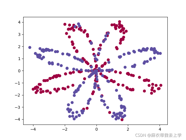
  以上就是我们这次作业需要使用的数据集。

2.逻辑回归完成二分类

上一周作业中我们手撸了一遍逻辑回归代码，从激活函数到损失函数再到正向反向传播，逻辑回归模型可以看成是隐藏层数量为0的神经网络结构。python中其实已经提供了相关的机器学习库(==sklearn==)来帮助我们快速的建立逻辑回归模型，我们利用sklearn库建立逻辑回归模型来对我们生成的数据进行分类。

import sklearn
from planar_utils import load_planar_dataset, plot_decision_boundary
import matplotlib.pyplot as plt
import numpy as np

X, Y = load_planar_dataset()
clf = sklearn.linear_model.LogisticRegressionCV()
clf.fit(X.T, Y.T)

plot_decision_boundary(lambda x: clf.predict(x), X, Y)  # 绘制决策边界
plt.title("Logistic Regression")  # 图标题
LR_predictions = clf.predict(X.T)  # 预测结果
print("逻辑回归的准确性： %d " % float((np.dot(Y, LR_predictions) +
                               np.dot(1 - Y, 1 - LR_predictions)) / float(Y.size) * 100) +
      "% " + "(正确标记的数据点所占的百分比)")

  结果如下：

  利用matplotlib绘制逻辑回归的决策边界。

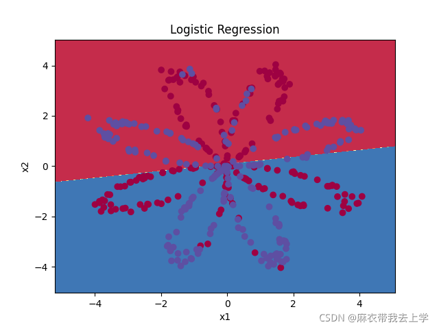
  从结果可以看出逻辑回归模型表现效果很差，也可以认为隐藏层数量为0的神经网络结构表现效果较差。

3.构建隐藏层数量为1的神经网络

  根据题目要求，我们可以将神经网络设计为如下结构：

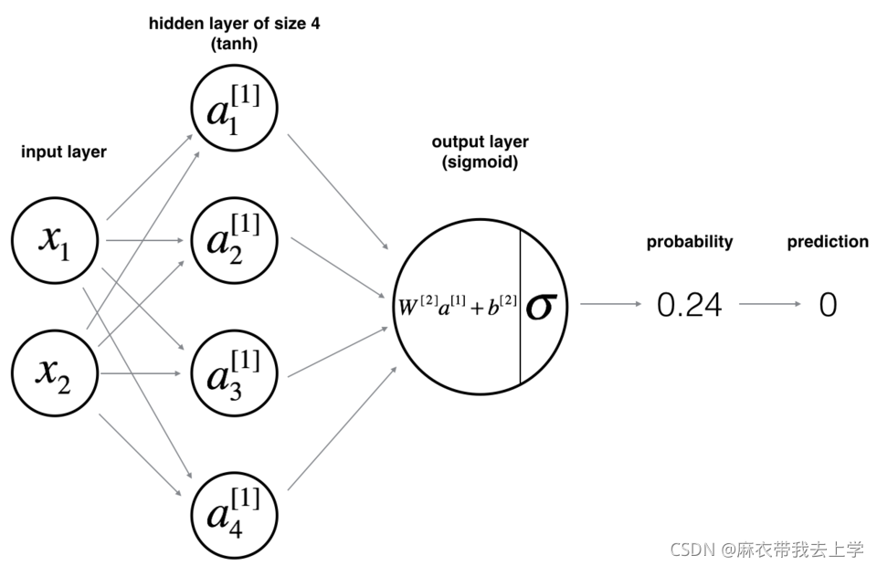
  隐藏层的神经单元使用的激活函数为 ==tanh== ，因为本次任务为二分类任务，输出层的激活函数可以为sigmoid。

3.1公式推导

  编程的重难点在于反向传播，作为初学者，加之这个神经网络结构比较简单，可以推导一下我们需要使用到的公式。

（在计算dz1的时候，W2需要转置，漏掉了个T）

3.2初始化

  我将单层神经网络封装成类 ==SimpleNN== 。

class SimpleNN(object):
    def __init__(self, input_layer, hidden_layer, output_layer):
        """
        初始化神经网络，这里的隐藏层只有一层
        :param input_layer: 输入层神经元个数
        :param hidden_layer: 隐藏层神经元个数
        :param output_layer: 输出层神经元个数
        """
        self.w = []
        self.b = []
        self.z = []
        self.a = []
        self.input_layer = input_layer
        self.hidden_layer = hidden_layer
        self.output_layer = output_layer
        self.initialize_parameters()

  隐藏层层数的设置默认为1层，没有考虑其他情况。需要注意的是，在正向传播时我们需要保存每一层 ==a== 和 ==z== 的计算结果，这也是视频中说的 ==cache== 。

  当我们获得了各层的参数时，可以对 ==w== 和 ==b== 进行初始化。

    def initialize_parameters(self):
        w1 = np.random.randn(self.hidden_layer, self.input_layer)
        w2 = np.random.randn(self.output_layer, self.hidden_layer)

        assert (w1.shape == (self.hidden_layer, self.input_layer))
        assert (w2.shape == (self.output_layer, self.hidden_layer))

        self.w = [w1, w2]

        b1 = numpy.zeros(shape=(self.hidden_layer, 1))
        b2 = numpy.zeros(shape=(self.output_layer, 1))

        assert (b1.shape == (self.hidden_layer, 1))
        assert (b2.shape == (self.output_layer, 1))

        self.b = [b1, b2]

3.3 激活函数

  隐藏层的激活函数为tanh，numpy库有自带的函数完成tanh函数功能。sigmoid函数需要自己编写。

    def sigmoid(self, z):
        """
        sigmoid激活函数，用于output层
        :param z: 输入
        :return:
        """
        return 1 / (1 + np.exp(-z))

  接下来可以根据计算顺序来设计相应的函数。

3.4正向传播

  正向传播比较容易实现。

 def forward(self, X):
        """
        前向传播
        :param X: 样本集
        :return:
        """
        m = X.shape[1]
        Z1 = np.dot(self.w[0], X) + self.b[0]
        A1 = np.tanh(Z1)

        Z2 = np.dot(self.w[1], A1) + self.b[1]
        A2 = self.sigmoid(Z2)

        self.z = [Z1, Z2]
        self.a = [X, A1, A2]

3.5 反向传播

    def backward(self, Y, learning_rate):
        """
        反向传播
        :param Y: 实际标签值
        :param learning_rate: 学习率
        :return:
        """
        sample_num = Y.shape[1]
        dZ2 = self.a[2] - Y
        dW2 = (1 / sample_num) * np.dot(dZ2, self.a[1].T)
        db2 = (1 / sample_num) * np.sum(dZ2, axis=1, keepdims=True)

        dZ1 = np.multiply(np.dot(self.w[1].T, dZ2), 1 - np.power(self.a[1], 2))
        dW1 = (1 / sample_num) * np.dot(dZ1, self.a[0].T)
        db1 = (1 / sample_num) * np.sum(dZ1, axis=1, keepdims=True)

        self.w[0] = self.w[0] - learning_rate * dW1
        self.w[1] = self.w[1] - learning_rate * dW2

        self.b[0] = self.b[0] - learning_rate * db1
        self.b[1] = self.b[1] - learning_rate * db2

  注意有的地方用的是点乘np.dot有的地方是np.multiply().

3.6 计算loss

    def compute_loss(self, A, Y):
        """
        计算损失函数
        :param A: 预测结果
        :param Y: 实际结果
        :return:
        """
        m = Y.shape[1]
        total_loss = (-1) * np.multiply(Y, np.log(A)) + np.multiply((1 - Y), np.log(1 - A))
        cost = (1 / m) * np.sum(total_loss)
        cost = float(np.squeeze(cost))
        assert (isinstance(cost, float))

        return cost

3.7 预测函数

    def predict(self, X):
        """
        预测函数
        :param X: 输入数据
        :return: 
        """
        self.forward(X)
        return np.round(self.a[2])

3.8 主控函数

    def nn_model(self, X, Y, learning_rate, iterations):
        """
        主控函数
        :param X: 输入样本
        :param Y: 实际标签值
        :param learning_rate: 学习率
        :param iterations: 迭代次数
        :return:
        """
        for i in range(0, iterations):
            self.forward(X)
            self.backward(Y, learning_rate)
            cost = self.compute_loss(self.a[2], Y)

4 运行

 X, Y = load_planar_dataset()
    nn = SimpleNN(2, 4, 1)
    nn.nn_model(X, Y, iterations=10000, learning_rate=0.5)
    # 绘制边界
    plot_decision_boundary(lambda x: nn.predict(x.T), X, Y)
    plt.title("Decision Boundary for hidden layer size " + str(4))
    plt.show()

    predictions = nn.predict(X)
    print('准确率: %d' % float((np.dot(Y, predictions.T) + np.dot(1 - Y, 1 - predictions.T)) / float(Y.size) * 100) + '%')

  运行结果：

  绘制决策边界：

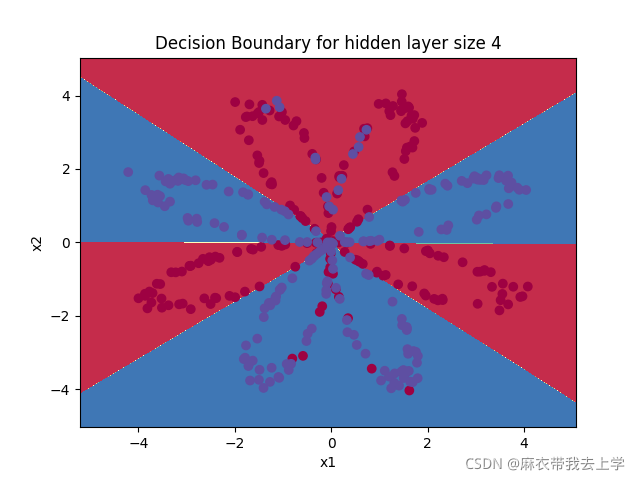
  可以看出增加一层隐藏层后，效果增加明显。

总结

  具体代码已经放入百度网盘中，提取码：ck6t。代码质量不是太高，请见谅。